In this post I will make the case that Bayesian models are much more intuitive than Frequentist models when it comes to parametrisation. Since Bayesian statistics consider data fixed and parameters as random, the resulting marginal posteriors can be interpreted and compared as such. In contrast, since Frequentist statistics consider parameters fixed and data random, inference of parameter estimates require all kinds of statistical tests, p-values, confidence intervals, corrections etc. which do not have very intuitive interpretation making comparison and joint considerations complicated.

To illustrate the intuitiveness and related problems with parameter interpretation, I will take a (in my opinion) well conducted Frequentist analysis and replicate it with Bayesian methods. To this end, I will be replicating the oil market model from Lütkepohl et al. (2020). They develop a formal statistical test for analysing the strength of identification in heteroskedastic VARs with two volatility states and demonstrate its use with the Kilian (2009) oil market model (I even used this in my master’s thesis).

For the sake of briefness, I won’t be going through the modelling details (I will try to put a full Bayesian cookbook out in the near future). However, as the main interest of this post is the strength of identification through heteroskedasticity, I will briefly go through the premises.

In the current setup, it is assumed that there is a change in the shock variances at some, predetermined point. We normalise the variance of the first volatility regime as unity. Thus the second regime variances can be interpreted in relative terms to the first. If at most one of the shocks is homoskedastic and the relative variances of regime two are unique from each other (without this shocks cannot be separated and thus not identified by their statistical properties), the structural parameters are identified. Thus, the question boils down to showing sufficient evidence on the uniqueness of the second regime variances.

Following the authors, I will include three lags and a constant term, while the volatility break is set to October 1987. In order to make the comparison as straightforward as possible, I will impose uninformative priors on all parameters, although in general I would not recommend the use of uninformative priors without a clear reasoning. Note also, that I am parametrising the model directly in the structural form, so no decomposing of reduced form error covariance matrix etc. The only regularisation is done in respect of the diagonal of the impact matrix, which is constrained to be positive.

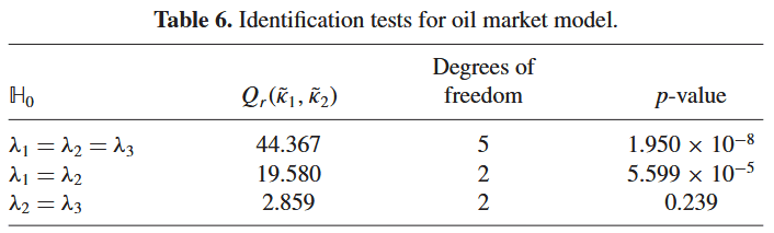
The authors run their tests on the identified variance parameters, results of which can be seen below. As can be seen, the results seem to indicate identification for at least one of the shocks. There are of course some caveats. First, as is well known (though often forgotten in practice) running several hypothesis tests at the same time raises multiple comparisons problems. In this particular case, the p-values for the first two tests are so small that it is probably not a concern for their validity. For the last test, this is something to keep in mind. The second caveat comes from the power of any test used. Through simulations, the authors find that the test tends to have lower power than intended i.e. a higher than intended probability of failing to reject the null when appropriate. On the other hand, their model is fairly small with a comparatively long sample size which should counter this. All in all, there seems to be quite clear evidence for the shock with largest variance being identified with the identification between the second and the third not being identified though some questions are raised.

So how does my Bayesian model answer the question about identification? In short, all of the parameters are distinct and non-unity, as can be seen from the figure below. End of the story, good night.

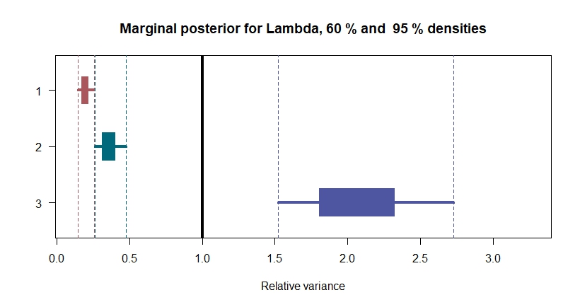
Well, a couple of notes can be made. First of course, note that where as the norm followed by the authors is to order the shocks from largest to smallest in terms of second regime variance, I have done it the other way around. This is purely due to convenience due to the built in function in Stan doing it this way. It does not affect the results of course. Note also, that despite being hard to see from the figure, the lines of the first and second shock do not cross: the 95% densities are distinct (if one chooses to care specifically about such an arbitrary number), though only barely. As such, it indicates full identification without all the questions and caveats of a Frequentist treatment.

Summa summarum: I think the biggest practical (although I could ramble for ages about the more philosophical side of things) advantage of Bayesian modelling is the fact that you get explicit probability distributions for estimated parameters, which makes interpretation so much easier. This is in contrast to the Frequentist side of things, where it is easy to get stuck on all kinds of questions about multiple comparisons problems and test power and size (and if you’re not, you’re probably misinterpreting your model output).

Not having to focus on the interpretation of your model output gives you time to focus on actually important things like model specification and priors.

This is of course as long as you don’t do something extremely stupid like forget that Bayesian treatment is all about taking into consideration all the uncertainty i.e. integrating over the whole parameter space.

P.S. Coding was done in R utilising Stan.