In their working paper, Bergholt et. al (2024) (hence “Authors”) illustrate that due to the estimation uncertainty of the constant (or in general all exogenous) term the historical decompositions built around such constant terms are prone to large quantitative and qualitative variation making them unreliable for inferential purposes. In this post I will briefly note that their conclusions are based on faulty premises stemming from incorrect practices regarding Bayesian estimation of vector autoregressions (VAR). Even though their case and solutions are (according to Mr. Canova) based on commonplace practices, the answer should not be to patch up incorrect inferential approaches but to do the inference correctly in the first place.

The illustrative starting place for the Authors is a bivariate VAR including the log differences of US GDP and GDP deflator from 1983Q1 to 2022Q4. The model is estimated with a constant and four lags. The estimated parameter space is set up by a diffuse prior on both the VAR coefficients and the covariance matrix and a Gaussian likelihood. As is well known, using a stacked form for the VAR equation this results in an analytical expression for the posterior distribution following

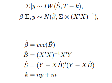
For details see e.g. the treatment of Silvia Miranda Agrippino and Giovanni Ricco. Importantly, one can then draw samples from these marginal densities. Note also, that due to the diffuse prior being uninformative and flat over the real space, the mean (and due to the Gaussian nature of it the median) of the marginal posterior distribution of any coefficient is its ordinary least squares (OLS) estimate.

The Authors then go on to take 1000 draws from this posterior and identify them with standard sign restrictions: aggregate supply shocks raise growth and lower inflation, aggregate demand shocks raise growth and inflation. To estimate historical decompositions they then pick the so-called Fry-Pagan draw as their point estimate. This is the single draw that produces impulse responses closest to the pointwise median impulse responses (the pointwise median, in general, does not correspond to any single model and set of coefficients as horizons are calculated by iterating the impact effect). They also take the second and third closest draws noting that these produce almost identical impulse responses. The reader is referred to the original article to observe these.

When historical decompositions of inflation are estimated for these three draws, the picture becomes very different. Indeed, the decompostions estimated by the Authors from these three draws do not even agree whether supply or demand factors were the main driver of the 2022 inflation surge. The problem is identified as originating from the uncertainty of the constant term estimate, which differs wildly from draw to draw. To solve this, the Authors propose to use a single-unit-root prior to shrink the estimate for the constant term to its unconditional mean.

There are several problems here. First, while natural in the context of the diffuse prior where the likelihood fully dictates the posterior, the shrinkage of the constant becomes conceptually problematic when any type of informative prior is considered. Second, and more importantly, it is based on an incorrect application of Bayesian methods in the first place. Individual draws from the posterior are just random draws. Only together do they present themselves as the whole joint posterior distribution.

To illustrate this, we start by noting that the Fry-Pagan draw is defined by the impulse responses which in turn are not affected by the exogenous part of the model. In this sense, after picking the draw, we can treat the lag coefficients as “known” as we have considered them and the constant coefficients as “unknown” as we have not considered them. Thus, we can arrange the block of VAR coefficients of the posteriors analytical expression into two blocks, the first containing the lag coefficients of the Fry-Pagan draw and the second the constant coefficients of it. We get:

where the Kronecker product of the original expression has been reformed and divided accordingly. As the first block is known, for the second we get:

Thus, it is easy to see that any Fry-Pagan-type draw will have its constant coefficients be random draws from a Gaussian distribution with mean at original posterior mean and variance diminished from it according to the already known coefficients. This is also why the single-unit-root prior works as a patchwork solution in the context of the diffuse prior: it simply shrinks the expected distance of an arbitrary draw to the OLS estimate which one would like to acquire anyway in this context.

So why fixate on an arbitrary random draw and not, say, the means of the marginal posterior distributions (towards which the draw is shrunk anyway)? The Authors and apparently a sizable part of the scientific community seem to confuse individual draws with candidate models. This of course, is not the case. Individual draws are indeed, despite being conditionally drawn, still random draws. Bayesian estimation does not concern with random draws, it concerns with probability distributions in the form of the posterior. Random draws are simply a tool to uncover this distribution.

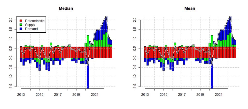
So how should the historical decompositions be estimated and how does the correct procedure measure up? In line with Bayesian inference, we would naturally want a posterior for the historical decomposition itself. This can be done by calculating the historical decomposition for every identified posterior draw and only then taking the mean, median or whatever point estimate seems appropriate for each individual element. In what follows I have done exactly this and estimated the historical decomposition for US inflation. The model is estimated with a diffuse prior and same specifications as by the Authors, but the historical decomposition is derived as I just described. As we can see from the picture below, the results are practically identical to the one by the Authors using the single-unit-root prior. No problems with the constant term, when the point estimate is drawn correctly in textbook fashion.

In the spirit of not providing prior information nor treating the posterior correctly one could also ask why even bother with Bayesian estimation? Why not just estimate the reduced form VAR with OLS, then draw 1000 candidates for identification with standard sign restrictions, take the mean or median from these and calculate the historical decomposition? Well, below I have done just that and the results, unsurprisingly are basically the same. Again, no problems with the constant term.

The Frequentist school is based on the philosophical idea of estimating the “true” point value of the parameter of interest from a sample. As such, providing optimal point estimates is what Frequentist methods are designed to do. The Bayesian school is based on the philosophical idea of estimating parameter uncertainty under the available information. As such, Bayesian methods are designed to provide optimal estimates for such a distribution. Sampling or simulating by Markov chains are tools used in Bayesian statistics to jointly estimate this distribution of interest. Confusing such samples with individual point estimates will thus lead to faulty inference. Note that this is not even a philosophical point, just an observation on how different methods are based on different principles, and will crumble if these principles are not understood and confused.

In summary, the problem contemplated by the Authors does not lie in econometric methods. These methods work just fine as they already are and do not require new gimmicks in order to be useful. Thus there is no problem with estimating historical decompositions in the first place. The problem lies in treating these models in a way they were never designed to be treated with.

According to Mr. Canova this kind of an approach is widespread. Why? I can only speculate. Maybe people used to Frequentis models find it hard to conceptualize distributions and the fact that point estimates have to be defined by themselves rather than given by statistical software (thus the potential confusing of individual posterior samples with candidate point estimates). Maybe coding these models properly takes more effort and is thus avoided. Personally, I do not see this as an excuse that warrants patchwork solutions. The real solution is to conduct scientific research properly or make way for those who will.

Especially since coding this is not really that hard.

P.S. The comments attributed to Mr. Fabio Canova are from a seminar hosted by him at the Bank of Finland in the summer of 2024, which I had the privilege and pleasure of attending to.

P.P.S. All programming was done with no dedicated attention to code optimization using only base libraries of R. All parts of the programming were run in a matter of seconds.